While mathematical expressions are important in any programming language, the topic of math functions addresses not just the algorithms themselves, but the design of custom functions within Python.
Many of you reading this article are likely to be technical professionals working in a technical setting. Therefore, every one of you has likely used a math function at some point in your life. One of the earliest examples I can personally recall was learning the slope-intercept form of a line in algebra:
$$y=m \cdot x+b$$
More formally written with y as “a function of x”:
$$f(x)=m \cdot x+b$$
What is a Function?
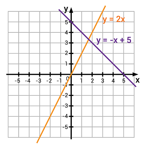
As a student, some of the broader concepts surrounding functions did not click until much later in my adult years. Particularly, this y = mx + b function describes a relationship between two variables in which the change of one is a direct, proportional change as a result of the other.
The input variable, x, drives the output of the dependent variable y. Furthermore, the sheer volume of homework problems and tests surrounding this equation proved its robust reusability across a wide range of linear equations. It made linear equations easier to work with and less of a manual task through the structured, repeatable form of the equation.
Python functions are similar to the slope-intercept linear equation we grew up with in algebra. It accepts input variables or arguments to produce an output or perform a task. They both serve a specific, targeted task and are highly repeatable.

Figure 1. Slope intercept form of linear equations with plotted lines.
Built-In Functions
The first kind of functions in Python are those that are built right into the language. They are included with the initial installation of Python and do not require a network connection or import statement to use (more on that ‘import’ statement later).
We’ll test out a few of these built-in numeric functions on the following sample list of process temperature values:
max()
The max function returns the largest value in the list.
Output:
66.23 Process finished with exit code 0
min()
Likewise, the min function returns the smallest value in the list.
Output:
23.323 Process finished with exit code 0
These are simple functions where the argument we supplied to the function was an iterable, the list of process temperature values. However, functions can be more complex and versatile to accept various types of arguments as well as default states.
Arguments
There are two main forms of arguments that can be supplied to a function: positional and keyword arguments.
Positional
Positional arguments are commonly used in Python functions. The function differentiates arguments supplied to it based on the order or position in which the arguments are provided.
This is better shown through use of the built-in pow() function which raises a provided number to the power of another. Let’s square the first temperature value in the list or raise to the power of 2:
Output:
543.9623290000001 Process finished with exit code 0
The defined positional arguments for the pow function appear as such:
Keyword
Another common argument type is keyword arguments. These arguments must always follow positional arguments. The value for the argument must be explicitly assigned to the keyword in order to pass to the function. For example, the pow() function has a keyword argument mod which follows the base and exp positional arguments. Calling the ‘help’ function on the pow function we can view the keyword argument:
Output:
pow(base, exp, mod=None) Equivalent to base**exp with 2 arguments or base**exp % mod with 3 arguments Some types, such as ints, are able to use a more efficient algorithm when invoked using the three argument form.
Notice how the mod keyword argument is assigned a default value of None? This is the reason we did not need to provide a value to mod in the prior positional argument section. However, we will override the None value with a modulus of 2 in this example. We will also round the temperature value to a whole integer since the pow function with a modulus defined can only accept all three arguments as integers:
Output:
1 Process finished with exit code 0
Custom Functions
So far, we have only been using functions that have already been built and pre-defined, but we can also build our own. A great example of a custom solution might be the slope-intercept linear form that opened this article.
With custom functions, we must first create or define the function prior to using it. Function definitions begin with a def keyword followed by function name and a colon. The nested body of the function contains a docstring which describes the inputs, outputs, and what the function does. Any uncommented code below the docstring drives the action of the function.
At the end of the function, a return keyword indicates what value(s) the function gives upon completion. Let’s take a look at the definition below:
Running this block of code will do nothing; it simply defines a function within the script. We must call the function and pass any necessary arguments in order to trigger any action:
Output:
11 Process finished with exit code 0
With this new skill, it gives us a way to distinguish between ‘out-of-the-box’ versus customized solutions. We would opt for the built-in solution if at all possible, but custom functions can help us define an algorithm for virtually any scenario.
Putting the ‘Fun’ in Functions
There is so much to cover in functions, we have barely scratched the surface! We’ll spend another article on functions before proceeding with further topics.
Copyright Statement: The content of this website is intended for personal learning purposes only. If it infringes upon your copyright, please contact us for removal. Email: [email protected]
